Plots and Data Summaries

Load data

In [1]:

library(tidyverse)

── Attaching core tidyverse packages ──────────────────────── tidyverse 2.0.0 ──
✔ dplyr     1.1.4     ✔ readr     2.1.5
✔ forcats   1.0.0     ✔ stringr   1.5.1
✔ ggplot2   3.5.1     ✔ tibble    3.2.1
✔ lubridate 1.9.4     ✔ tidyr     1.3.1
✔ purrr     1.0.4     
── Conflicts ────────────────────────────────────────── tidyverse_conflicts() ──
✖ dplyr::filter() masks stats::filter()
✖ dplyr::lag()    masks stats::lag()
ℹ Use the conflicted package (<http://conflicted.r-lib.org/>) to force all conflicts to become errors

library(bruneimap)

Loading required package: sf
Linking to GEOS 3.11.0, GDAL 3.5.3, PROJ 9.1.0; sf_use_s2() is TRUE

library(gt)
library(gtsummary)
library(lubridate)
library(GGally)

Registered S3 method overwritten by 'GGally':
  method from   
  +.gg   ggplot2

here::i_am("notebooks/data.R")

here() starts at /Users/haziqj/github_local/house-data

# Main data set
hsp <- 
  read_csv(here::here("data/hspbn_2025-03-03.csv")) |>
  mutate(
    type = factor(type, levels = c("Detached", "Semi-Detached", "Terrace",
                                   "Apartment", "Land")),
    tenure = factor(tenure, levels = c("Freehold", "Leasehold", "Strata")),
    status = factor(status, levels = c("Proposed", "Under Construction", "New", "Resale")),
    date = as.Date(date, format = "%d/%m/%y"),
    quarter = zoo::as.yearqtr(quarter)
  )

Rows: 31116 Columns: 18
── Column specification ────────────────────────────────────────────────────────
Delimiter: ","
chr  (10): quarter, kampong, mukim, district, type, tenure, status, agent, s...
dbl   (7): id, price, plot_area, floor_area, storeys, beds, baths
date  (1): date

ℹ Use `spec()` to retrieve the full column specification for this data.
ℹ Specify the column types or set `show_col_types = FALSE` to quiet this message.

# RPPI from BDCB
rppi <- 
  read_csv(here::here("data/rppi.csv")) |>
  mutate(
    quarter = zoo::as.yearqtr(quarter),
    rppi = rppi / 100
  )

Rows: 39 Columns: 2
── Column specification ────────────────────────────────────────────────────────
Delimiter: ","
chr (1): quarter
dbl (1): rppi

ℹ Use `spec()` to retrieve the full column specification for this data.
ℹ Specify the column types or set `show_col_types = FALSE` to quiet this message.

# To create median price per square foot, need to filter out "Land" types as
# well as missing property types. Then create an "Overall" type.
hsp_all <- 
  bind_rows(
    hsp, 
    mutate(hsp, type = "Overall")
  ) |> 
  arrange(date) 

# Create a median price per square foot index
hsp_rppi <-
  slider::slide_period_dfr(hsp, hsp$date, "month", \(df) {
    df |>
      filter(type != "Land") |>
      drop_na(floor_area) |>
      summarise(
        quarter = first(quarter),
        price = median(price, na.rm = TRUE),
        # plot_area = median(plot_area, na.rm = TRUE),
        floor_area = median(floor_area, na.rm = TRUE)
      )
  }, .before = 1, .after = 1) |>
  summarise(across(price:floor_area, \(x) median(x, na.rm = TRUE)), .by = quarter) |> 
  drop_na(quarter) |>
  mutate(
    price_per_sqft = price / floor_area,
    index = price_per_sqft / price_per_sqft[quarter == "2015 Q1"],
  ) |>
  right_join(rppi, by = join_by(quarter)) 

rppi_mae <-
  hsp_rppi |>
  summarise(
    rmse = (mean( abs(rppi - index) ^ 1)),
    range = max(c(rppi)) - min(c(rppi)),
    mean = mean(c(rppi)),
    sd = sd(c(rppi))
  ) |>
  unlist()

# (rmse <- as.numeric(rppi_mae[1]))
# (nmae <- (rppi_mae[1] / rppi_mae[-1])[2])

# Create an sf data frame for plotting Brunei map
hsp_mkm <-
  hsp |>
  summarise(
    price = median(price, na.rm = TRUE, trim = 0.05),
    .by = mukim
  ) |>
  left_join(x = bruneimap::mkm_sf, by = join_by(mukim)) 

Summary of variables

In [2]:

In [3]:

hsp |>
  mutate(
    price = price / 1000,
    storeys = factor(
      ifelse(storeys >= 3, "3+", as.character(storeys)),
      levels = c("1", "2", "3+")
    ),
    district = gsub("Brunei Muara", "Brunei-Muara", district),
    district = factor(district, levels = c("Brunei-Muara", "Belait", "Tutong", "Temburong"))
  ) |>
  tbl_summary(
    include = c(price:baths),
    by = district,
    missing = "no", 
    type = all_continuous() ~ "continuous2",
    statistic = list(
      all_continuous2() ~ c("{mean} ({sd})", Range = "{min} - {max}", "{median} ({p25}, {p75})")
    ),
    label = list(
      price = "Price (BND 1,000)",
      type = "Property type",
      plot_area = "Plot area (acres)",
      floor_area = "Floor area (sq. ft.)",
      storeys = "Number of storeys",
      status = "Development status",
      tenure = "Land tenure",    
      beds = "Number of bedrooms",
      baths = "Number of bathrooms"
    ),
    digits = list(
      baths = 1,
      beds = 1
    )
  ) |>
  add_overall() |>
  add_n() |>
  modify_header(label ~ "**Variable**") |>
  as_gt()

Summary of housing data.

Variable	N	Overall N = 31,1161	Brunei-Muara N = 28,5701	Belait N = 1,4841	Tutong N = 7671	Temburong N = 2951
Price (BND 1,000)	31,116
Mean (SD)		340 (381)	340 (393)	372 (208)	259 (87)	421 (324)
Min - Max		70 - 13,800	70 - 13,800	98 - 2,800	116 - 680	118 - 1,800
Median (Q1, Q3)		288 (230, 380)	285 (230, 380)	320 (268, 400)	245 (198, 310)	390 (250, 430)
Property type	27,231
Detached		17,416 (64%)	16,307 (65%)	520 (42%)	509 (74%)	80 (56%)
Semi-Detached		3,823 (14%)	3,591 (14%)	97 (7.8%)	128 (19%)	7 (4.9%)
Terrace		4,449 (16%)	4,134 (16%)	213 (17%)	48 (7.0%)	54 (38%)
Apartment		1,527 (5.6%)	1,106 (4.4%)	414 (33%)	4 (0.6%)	3 (2.1%)
Land		16 (<0.1%)	11 (<0.1%)	4 (0.3%)	1 (0.1%)	0 (0%)
Land tenure	12,877
Freehold		9,296 (72%)	8,405 (76%)	368 (33%)	381 (80%)	142 (97%)
Leasehold		2,783 (22%)	2,221 (20%)	467 (41%)	91 (19%)	4 (2.7%)
Strata		798 (6.2%)	504 (4.5%)	291 (26%)	3 (0.6%)	0 (0%)
Development status	22,481
Proposed		4,004 (18%)	3,660 (18%)	103 (8.8%)	197 (33%)	44 (31%)
Under Construction		9,420 (42%)	8,600 (42%)	535 (46%)	244 (41%)	41 (29%)
New		7,724 (34%)	7,122 (35%)	413 (35%)	132 (22%)	57 (40%)
Resale		1,333 (5.9%)	1,186 (5.8%)	120 (10%)	26 (4.3%)	1 (0.7%)
Plot area (acres)	23,368
Mean (SD)		0.16 (0.12)	0.15 (0.11)	0.19 (0.15)	0.18 (0.17)	0.23 (0.21)
Min - Max		0.01 - 2.00	0.01 - 1.69	0.01 - 1.01	0.04 - 2.00	0.05 - 0.96
Median (Q1, Q3)		0.13 (0.08, 0.19)	0.13 (0.08, 0.19)	0.13 (0.06, 0.27)	0.14 (0.10, 0.21)	0.16 (0.13, 0.26)
Floor area (sq. ft.)	16,665
Mean (SD)		2,602 (1,047)	2,629 (1,062)	2,423 (913)	2,133 (651)	2,786 (751)
Min - Max		500 - 14,411	500 - 14,411	600 - 7,500	1,093 - 7,000	950 - 3,700
Median (Q1, Q3)		2,427 (2,000, 3,000)	2,465 (2,000, 3,000)	2,218 (1,800, 2,800)	2,013 (1,826, 2,450)	3,016 (2,790, 3,229)
Number of storeys	13,644
1		1,700 (12%)	1,462 (12%)	160 (35%)	71 (17%)	7 (4.2%)
2		11,266 (83%)	10,493 (83%)	280 (61%)	348 (83%)	145 (87%)
3+		678 (5.0%)	642 (5.1%)	19 (4.1%)	2 (0.5%)	15 (9.0%)
Number of bedrooms	26,631
Mean (SD)		4.2 (0.9)	4.2 (0.9)	4.0 (1.1)	3.9 (0.7)	4.7 (1.0)
Min - Max		0.0 - 12.0	0.0 - 12.0	1.0 - 10.0	2.0 - 7.0	2.0 - 7.0
Median (Q1, Q3)		4.0 (4.0, 5.0)	4.0 (4.0, 5.0)	4.0 (3.0, 4.0)	4.0 (3.0, 4.0)	5.0 (4.0, 5.0)
Number of bathrooms	19,694
Mean (SD)		3.7 (1.2)	3.7 (1.2)	3.3 (1.1)	3.3 (1.0)	3.2 (1.5)
Min - Max		1.0 - 11.0	1.0 - 11.0	1.0 - 8.0	1.0 - 7.0	1.0 - 5.0
Median (Q1, Q3)		3.0 (3.0, 4.0)	3.0 (3.0, 4.0)	3.0 (3.0, 4.0)	3.0 (2.0, 4.0)	2.0 (2.0, 5.0)
1 n (%)

Correlations

In [4]:

my_fn <- function(data, mapping, method = "lm", ...) {
  ggplot(data = data, mapping = mapping) + 
    geom_point(alpha = 0.5) + 
    geom_smooth(method = method, formula = y ~ x, se = FALSE,
                col = RColorBrewer::brewer.pal(3, "Set1")[2], ...)
}

pm <-
  hsp |>
  mutate(
    logprice = log(price),
    price = price / 1000
  ) |>
  select(
    `Plot area` = plot_area,
    `Floor area` = floor_area,
    Beds = beds,
    Baths = baths,
    `Price (BND 1,000)` = price,
    `Log Price` = logprice
  ) |>
  ggpairs(
    progress = FALSE,
    lower = list(continuous = my_fn)
  ) +
  theme_bw() +
  scale_x_continuous(labels = scales::number) +
  scale_y_continuous(labels = scales::number) +
  theme(
    axis.text.x = element_text(angle = 45, hjust = 1)
  )

Warning in ggally_statistic(data = data, mapping = mapping, na.rm = na.rm, :
Removed 16641 rows containing missing values

Scale for x is already present.
Adding another scale for x, which will replace the existing scale.

Warning in ggally_statistic(data = data, mapping = mapping, na.rm = na.rm, :
Removed 10136 rows containing missing values

Scale for x is already present.
Adding another scale for x, which will replace the existing scale.

Warning in ggally_statistic(data = data, mapping = mapping, na.rm = na.rm, :
Removed 15292 rows containing missing values

Scale for x is already present.
Adding another scale for x, which will replace the existing scale.

Warning in ggally_statistic(data = data, mapping = mapping, na.rm = na.rm, :
Removed 14313 rows containing missing values

Scale for x is already present.
Adding another scale for x, which will replace the existing scale.

Warning in ggally_statistic(data = data, mapping = mapping, na.rm = na.rm, :
Removed 16516 rows containing missing values

Scale for x is already present.
Adding another scale for x, which will replace the existing scale.

Warning in ggally_statistic(data = data, mapping = mapping, na.rm = na.rm, :
Removed 11496 rows containing missing values

Scale for x is already present.
Adding another scale for x, which will replace the existing scale.

Warning in ggally_statistic(data = data, mapping = mapping, na.rm = na.rm, :
Removed 7748 rows containing missing values

Scale for x is already present.
Adding another scale for x, which will replace the existing scale.

Warning in ggally_statistic(data = data, mapping = mapping, na.rm = na.rm, :
Removed 14451 rows containing missing values

Scale for x is already present.
Adding another scale for x, which will replace the existing scale.

Warning in ggally_statistic(data = data, mapping = mapping, na.rm = na.rm, :
Removed 4485 rows containing missing values

Scale for x is already present.
Adding another scale for x, which will replace the existing scale.

Warning in ggally_statistic(data = data, mapping = mapping, na.rm = na.rm, :
Removed 11422 rows containing missing values

Scale for x is already present.
Adding another scale for x, which will replace the existing scale.

Warning in ggally_statistic(data = data, mapping = mapping, na.rm = na.rm, :
Removed 7748 rows containing missing values

Scale for x is already present.
Adding another scale for x, which will replace the existing scale.

Warning in ggally_statistic(data = data, mapping = mapping, na.rm = na.rm, :
Removed 14451 rows containing missing values

Scale for x is already present.
Adding another scale for x, which will replace the existing scale.

Warning in ggally_statistic(data = data, mapping = mapping, na.rm = na.rm, :
Removed 4485 rows containing missing values

Scale for x is already present.
Adding another scale for x, which will replace the existing scale.

Warning in ggally_statistic(data = data, mapping = mapping, na.rm = na.rm, :
Removed 11422 rows containing missing values

Scale for x is already present.
Adding another scale for x, which will replace the existing scale.
Scale for x is already present.
Adding another scale for x, which will replace the existing scale.
Scale for y is already present.
Adding another scale for y, which will replace the existing scale.
Scale for y is already present.
Adding another scale for y, which will replace the existing scale.
Scale for y is already present.
Adding another scale for y, which will replace the existing scale.
Scale for y is already present.
Adding another scale for y, which will replace the existing scale.
Scale for y is already present.
Adding another scale for y, which will replace the existing scale.
Scale for y is already present.
Adding another scale for y, which will replace the existing scale.
Scale for y is already present.
Adding another scale for y, which will replace the existing scale.
Scale for y is already present.
Adding another scale for y, which will replace the existing scale.
Scale for y is already present.
Adding another scale for y, which will replace the existing scale.
Scale for y is already present.
Adding another scale for y, which will replace the existing scale.
Scale for y is already present.
Adding another scale for y, which will replace the existing scale.
Scale for y is already present.
Adding another scale for y, which will replace the existing scale.
Scale for y is already present.
Adding another scale for y, which will replace the existing scale.
Scale for y is already present.
Adding another scale for y, which will replace the existing scale.
Scale for y is already present.
Adding another scale for y, which will replace the existing scale.
Scale for y is already present.
Adding another scale for y, which will replace the existing scale.
Scale for y is already present.
Adding another scale for y, which will replace the existing scale.
Scale for y is already present.
Adding another scale for y, which will replace the existing scale.
Scale for y is already present.
Adding another scale for y, which will replace the existing scale.
Scale for y is already present.
Adding another scale for y, which will replace the existing scale.
Scale for y is already present.
Adding another scale for y, which will replace the existing scale.

pm[6,5] <- pm[5, 6] <- NULL
pm

Warning: Removed 7748 rows containing non-finite outside the scale range
(`stat_density()`).

Warning: Removed 16641 rows containing non-finite outside the scale range
(`stat_smooth()`).

Warning: Removed 16641 rows containing missing values or values outside the scale range
(`geom_point()`).

Warning: Removed 14451 rows containing non-finite outside the scale range
(`stat_density()`).

Warning: Removed 10136 rows containing non-finite outside the scale range
(`stat_smooth()`).

Warning: Removed 10136 rows containing missing values or values outside the scale range
(`geom_point()`).

Warning: Removed 15292 rows containing non-finite outside the scale range
(`stat_smooth()`).

Warning: Removed 15292 rows containing missing values or values outside the scale range
(`geom_point()`).

Warning: Removed 4485 rows containing non-finite outside the scale range
(`stat_density()`).

Warning: Removed 14313 rows containing non-finite outside the scale range
(`stat_smooth()`).

Warning: Removed 14313 rows containing missing values or values outside the scale range
(`geom_point()`).

Warning: Removed 16516 rows containing non-finite outside the scale range
(`stat_smooth()`).

Warning: Removed 16516 rows containing missing values or values outside the scale range
(`geom_point()`).

Warning: Removed 11496 rows containing non-finite outside the scale range
(`stat_smooth()`).

Warning: Removed 11496 rows containing missing values or values outside the scale range
(`geom_point()`).

Warning: Removed 11422 rows containing non-finite outside the scale range
(`stat_density()`).

Warning: Removed 7748 rows containing non-finite outside the scale range
(`stat_smooth()`).

Warning: Removed 7748 rows containing missing values or values outside the scale range
(`geom_point()`).

Warning: Removed 14451 rows containing non-finite outside the scale range
(`stat_smooth()`).

Warning: Removed 14451 rows containing missing values or values outside the scale range
(`geom_point()`).

Warning: Removed 4485 rows containing non-finite outside the scale range
(`stat_smooth()`).

Warning: Removed 4485 rows containing missing values or values outside the scale range
(`geom_point()`).

Warning: Removed 11422 rows containing non-finite outside the scale range
(`stat_smooth()`).

Warning: Removed 11422 rows containing missing values or values outside the scale range
(`geom_point()`).

Warning: Removed 7748 rows containing non-finite outside the scale range
(`stat_smooth()`).

Warning: Removed 7748 rows containing missing values or values outside the scale range
(`geom_point()`).

Warning: Removed 14451 rows containing non-finite outside the scale range
(`stat_smooth()`).

Warning: Removed 14451 rows containing missing values or values outside the scale range
(`geom_point()`).

Warning: Removed 4485 rows containing non-finite outside the scale range
(`stat_smooth()`).

Warning: Removed 4485 rows containing missing values or values outside the scale range
(`geom_point()`).

Warning: Removed 11422 rows containing non-finite outside the scale range
(`stat_smooth()`).

Warning: Removed 11422 rows containing missing values or values outside the scale range
(`geom_point()`).

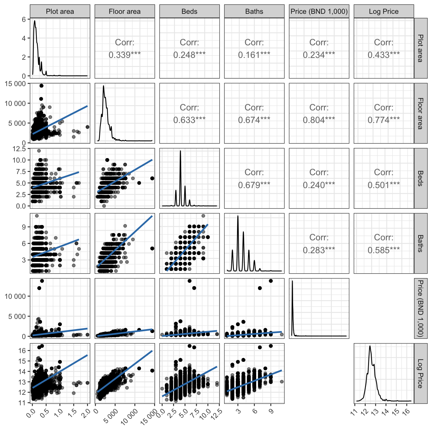
Pairwise correlation plot of continuous variables.

Data availability by year

In [5]:

In [6]:

hsp |>
  mutate(
    year = year(date),
    missing_price = is.na(price),
    missing_type = is.na(type),
    missing_tenure = is.na(tenure),
    missing_status = is.na(status),
    missing_plot_area = is.na(plot_area),
    missing_floor_area = is.na(floor_area),
    missing_storeys = is.na(storeys),
    missing_beds = is.na(beds),
    missing_baths = is.na(baths),
    missing_housechar = missing_plot_area & missing_floor_area & missing_beds & missing_baths,
    year = year(quarter),
  ) |>
  summarise(
    count = n(),
    spatial = length(unique(mukim)) / length(unique(hsp$mukim)),
    # price = sum(missing_price),
    type = sum(missing_type),
    house_char = sum(missing_housechar),
    source = list(unique(method)),
    .by = year
  ) |>
  mutate(
    `nat-archive` = map_chr(source, ~ ifelse("nat-archive" %in% .x, "✔", "")),
    `online-archive` = map_chr(source, ~ ifelse("online-archive" %in% .x, "✔", "")),
    `web-scrape` = map_chr(source, ~ ifelse("web-scrape" %in% .x | "web-scrape-llm" %in% .x, "✔", "")),
    llm = map_chr(source, ~ ifelse("web-scrape-llm" %in% .x, "✔", ""))
  ) |> 
  select(-source) |>
  mutate(across(type:house_char, \(x) x / count)) |>
  gt(rowname_col = "year") |>
  cols_align(
    align = "center",
    columns = `nat-archive`:llm
  ) |>
  tab_spanner(
    label = "Data source",
    columns = `nat-archive`:`web-scrape`
  ) |>
  tab_spanner(
    label = "Missing data severity",
    columns = type:house_char
  ) |>
  fmt_percent(
    spatial:house_char,
    decimals = 1
  ) |>
  cols_label(
    year ~ "Year",
    count ~ "Count",
    spatial ~ "Spatial coverage (mukim)",
    type ~ "Property Type",
    house_char ~ "Property Characteristics",
    `nat-archive` ~ "National Archive",
    `online-archive` ~ "Online Archive",
    `web-scrape` ~ "Web Scraping",
    llm ~ "LLM post-processing"
  ) |>
  grand_summary_rows(
    columns = count:house_char,
    fns = list(Mean = "mean"),
    fmt = list(
      ~ fmt_number(., decimals = 0, columns = "count"),
      ~ fmt_percent(., decimals = 1, columns = c("spatial", "type", "house_char"))
    )
  ) |>
  tab_footnote(
    footnote = paste0("Of Brunei’s 39 mukims, only 27 are considered transactable--excluding water villages and remote, non-developable areas."),
    locations = cells_column_labels(columns = spatial)
  ) |>
  tab_footnote(
    footnote = "Unknown property type.",
    locations = cells_column_labels(columns = type)
  ) |>
  tab_footnote(
    footnote = "Missing all of plot area, floor area, beds, and baths variables.",
    locations = cells_column_labels(columns = house_char)
  ) |>
  tab_options(
    quarto.disable_processing = TRUE,
    grand_summary_row.text_transform = "capitalize"
  ) 

Data availability by year.

	Count	Spatial coverage (mukim)1	Missing data severity		Data source			LLM post-processing
			Property Type2	Property Characteristics3	National Archive	Online Archive	Web Scraping
1993	400	33.3%	0.0%	19.0%	✔
1994	653	51.9%	65.8%	27.9%	✔
1995	668	70.4%	66.8%	21.3%	✔
1996	561	51.9%	69.7%	12.1%	✔
1997	385	51.9%	38.4%	26.8%	✔
1998	345	48.1%	36.8%	28.7%	✔
1999	317	51.9%	31.9%	26.2%	✔
2000	378	63.0%	0.8%	4.2%	✔
2001	342	63.0%	0.3%	2.3%	✔
2002	437	63.0%	0.0%	20.4%	✔
2003	449	66.7%	0.0%	13.4%	✔
2004	440	63.0%	0.0%	19.1%	✔
2005	493	66.7%	0.0%	13.2%	✔
2006	653	59.3%	0.2%	11.3%	✔
2007	638	55.6%	0.0%	12.9%	✔
2008	687	59.3%	0.3%	5.8%	✔
2009	531	51.9%	0.2%	4.0%	✔
2010	571	55.6%	0.0%	2.1%	✔
2011	594	55.6%	0.2%	10.1%	✔
2012	934	63.0%	8.0%	4.3%	✔		✔
2013	882	59.3%	2.9%	26.4%	✔	✔	✔
2014	709	66.7%	10.6%	8.0%		✔	✔
2015	868	66.7%	12.6%	6.3%		✔	✔
2016	1461	70.4%	13.6%	4.6%		✔	✔
2017	1638	70.4%	14.5%	4.5%		✔	✔
2018	2646	66.7%	17.6%	0.0%			✔
2019	3586	63.0%	15.9%	0.0%			✔
2020	1363	66.7%	10.4%	0.0%			✔	✔
2021	1115	77.8%	2.0%	0.0%			✔	✔
2022	1235	77.8%	3.6%	0.0%			✔	✔
2023	1593	77.8%	2.8%	0.0%			✔	✔
2024	2972	77.8%	4.6%	0.1%			✔	✔
2025	572	59.3%	14.7%	0.0%			✔	✔
mean	943	62.0%	13.5%	10.1%	—	—	—	—
1 Of Brunei’s 39 mukims, only 27 are considered transactable--excluding water villages and remote, non-developable areas.
2 Unknown property type.
3 Missing all of plot area, floor area, beds, and baths variables.

Spatial distribution

In [7]:

ggplot(hsp_mkm) +
  geom_sf(aes(fill = price), col = "gray50", linewidth = 0.5) +
  scale_fill_viridis_c(
    option = "cividis",
    na.value = "transparent",
    labels = scales::dollar,
    trans = scales::pseudo_log_trans(sigma = 0.001),
    name = "Median\nprice"
  ) +
  ggrepel::geom_label_repel(
    data = drop_na(hsp_mkm, price) |> 
      mutate(mukim = gsub("Mukim ", "", mukim)),
    aes(label = mukim, geometry = geometry),
    size = 2.7,
    stat = "sf_coordinates",
    max.overlaps = Inf,
    min.segment.length = 0,       
    segment.size = 0.3,           
    segment.curvature = 0.1,      
    force = 5                     
  ) +
  labs(x = NULL, y = NULL) +
  theme_bw()

Warning in st_point_on_surface.sfc(sf::st_zm(x)): st_point_on_surface may not
give correct results for longitude/latitude data

Spatial distribution of median property prices by mukim.

Price evolution

In [8]:

slider::slide_period_dfr(hsp_all, hsp_all$date, "month", \(df) {
  df |>
    filter(type != "Land") |>
    summarise(
      date = min(date), 
      price = median(price, na.rm = TRUE),
      plot_area = median(plot_area, na.rm = TRUE),
      floor_area = median(floor_area, na.rm = TRUE),
      .by = type
    )
}, .before = 18, .after = 6) |>
  distinct(date, type, .keep_all = TRUE) |> 
  mutate(
    price_per_sqft = price / floor_area,
    type = factor(type, levels = c("Detached", "Semi-Detached", "Terrace",
                                   "Apartment", "Overall")) 
  ) |>
  ggplot(aes(x = date, y = price_per_sqft, col = type)) +
  geom_line(aes(linewidth = type)) +
  scale_x_date(
    breaks = scales::breaks_width("1 year"), 
    labels = scales::label_date("%Y"),
    name = NULL
  ) +
  scale_y_continuous(
    labels = scales::dollar,
    name = "Price per square foot (BND)"
  ) +
  scale_colour_manual(values = c(RColorBrewer::brewer.pal(4, "Set1"), "black")) +
  scale_linewidth_manual(values = c(rep(0.6, 4), 1.2)) +
  labs(
    col = NULL,
    linewidth = NULL
    # caption = "Median smoothed prices using a 12-month rolling window."
  ) +
  theme_bw() +
  theme(
    axis.text.x = element_text(angle = 45, hjust = 1),
    legend.position = "top"
  ) 

Warning: Removed 20 rows containing missing values or values outside the scale range
(`geom_line()`).

Median smoothed prices per square foot by property type using a 24-month (8-quarter) rolling window.

RPPI Comparison

In [9]:

hsp_rppi |>  
  pivot_longer(c(index, rppi), names_to = "series", values_to = "value") |>
  ggplot(aes(x = quarter, y = value, col = series)) +
  geom_hline(yintercept = 1, linetype = "dashed") +
  geom_line(linewidth = 0.8) +
  scale_colour_brewer(palette = "Set1") +
  scale_y_continuous(labels = scales::percent, name = "Index") +
  zoo::scale_x_yearqtr(
    format = "%Y-Q%q", 
    expand = c(0, 0.1),
    name = NULL, 
    breaks = seq(2015, 2024.75, by = 0.25)
  ) +
  theme_bw() +
  theme(
    axis.text.x = element_text(angle = 45, hjust = 1),
    legend.position = "none"
  ) +
  geom_text(
    data = tibble(
      quarter = c(2024.3 + 0.25, 2024.3 + 0.25),
      series = c("index", "rppi"),
      value = c(0.941, 0.955) - 0.02,
      label = c("Median PPSF", "RPPI (BDCB)")
    ),
    aes(label = label),
    hjust = 0
  ) +
  coord_cartesian(xlim = c(2015, 2025.75))

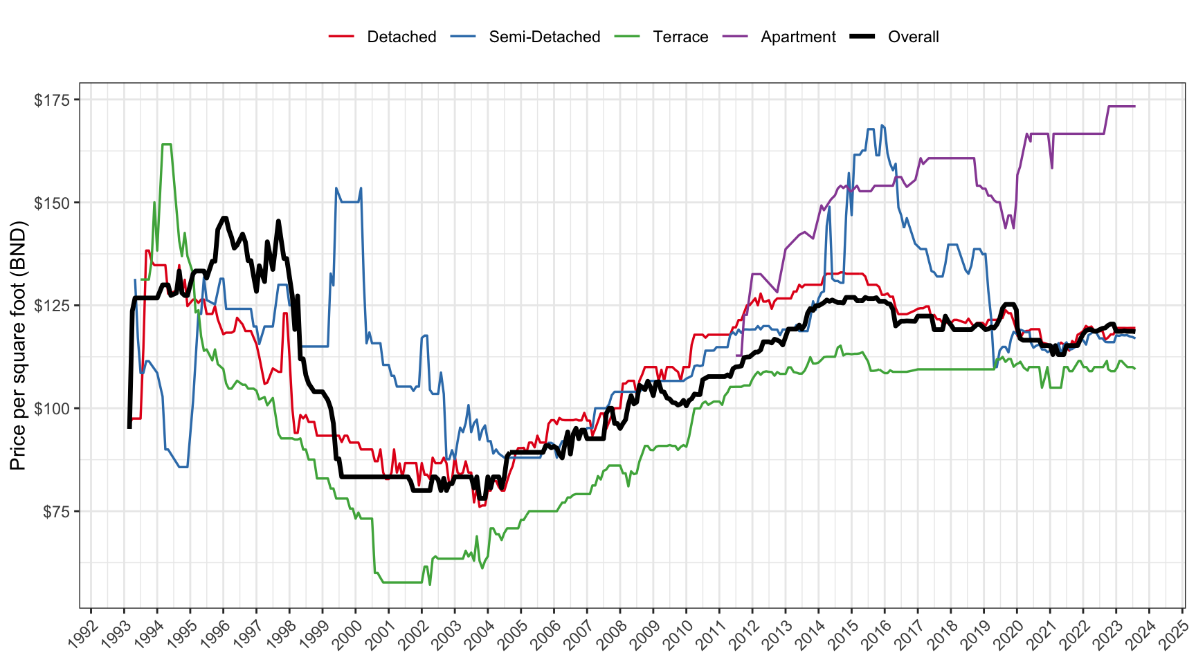
Comparison of quarterly median price per square foot indices (Median PPSF) and the official Residential Property Price Index (RPPI) from Brunei Darussalam Central Bank (BDCB).

LLM Test

In [10]:

load(here::here("experiments/llm_test.RData"))
p_llm_test

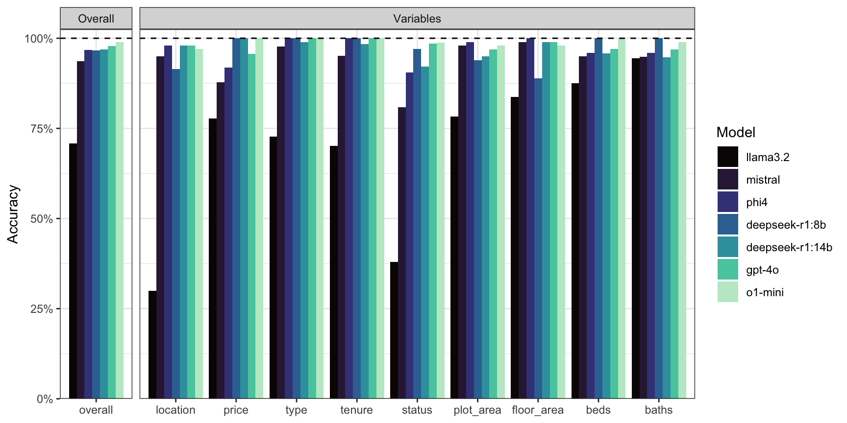
Comparison of data extraction accuracy across multiple LLM models on the test dataset. Each bar represents the percentage of correctly extracted fields for a given model.