Registered S3 method overwritten by 'GGally':
  method from
  +.gg   ggplot2
here::i_am("notebooks/data.R")
here() starts at /Users/haziqj/github_local/house-data
# Main data sethsp <-read_csv(here::here("data/hspbn_2025-03-03.csv")) |>mutate(type =factor(type, levels =c("Detached", "Semi-Detached", "Terrace","Apartment", "Land")),tenure =factor(tenure, levels =c("Freehold", "Leasehold", "Strata")),status =factor(status, levels =c("Proposed", "Under Construction", "New", "Resale")),date =as.Date(date, format ="%d/%m/%y"),quarter = zoo::as.yearqtr(quarter) )
Rows: 31116 Columns: 18
── Column specification ────────────────────────────────────────────────────────
Delimiter: ","
chr  (10): quarter, kampong, mukim, district, type, tenure, status, agent, s...
dbl   (7): id, price, plot_area, floor_area, storeys, beds, baths
date  (1): date

ℹ Use `spec()` to retrieve the full column specification for this data.
ℹ Specify the column types or set `show_col_types = FALSE` to quiet this message.
Rows: 39 Columns: 2
── Column specification ────────────────────────────────────────────────────────
Delimiter: ","
chr (1): quarter
dbl (1): rppi

ℹ Use `spec()` to retrieve the full column specification for this data.
ℹ Specify the column types or set `show_col_types = FALSE` to quiet this message.
# To create median price per square foot, need to filter out "Land" types as# well as missing property types. Then create an "Overall" type.hsp_all <-bind_rows( hsp, mutate(hsp, type ="Overall") ) |>arrange(date) # Create a median price per square foot indexhsp_rppi <- slider::slide_period_dfr(hsp, hsp$date, "month", \(df) { df |>filter(type !="Land") |>drop_na(floor_area) |>summarise(quarter =first(quarter),price =median(price, na.rm =TRUE),# plot_area = median(plot_area, na.rm = TRUE),floor_area =median(floor_area, na.rm =TRUE) ) }, .before =1, .after =1) |>summarise(across(price:floor_area, \(x) median(x, na.rm =TRUE)), .by = quarter) |>drop_na(quarter) |>mutate(price_per_sqft = price / floor_area,index = price_per_sqft / price_per_sqft[quarter =="2015 Q1"], ) |>right_join(rppi, by =join_by(quarter)) rppi_mae <- hsp_rppi |>summarise(rmse = (mean( abs(rppi - index) ^1)),range =max(c(rppi)) -min(c(rppi)),mean =mean(c(rppi)),sd =sd(c(rppi)) ) |>unlist()# (rmse <- as.numeric(rppi_mae[1]))# (nmae <- (rppi_mae[1] / rppi_mae[-1])[2])# Create an sf data frame for plotting Brunei maphsp_mkm <- hsp |>summarise(price =median(price, na.rm =TRUE, trim =0.05),.by = mukim ) |>left_join(x = bruneimap::mkm_sf, by =join_by(mukim))
Missing data patterns
Let’s take a look at the missing data patterns in the housing data. For simplicity, we focus on the year 2024 and houses in the Brunei-Muara district.
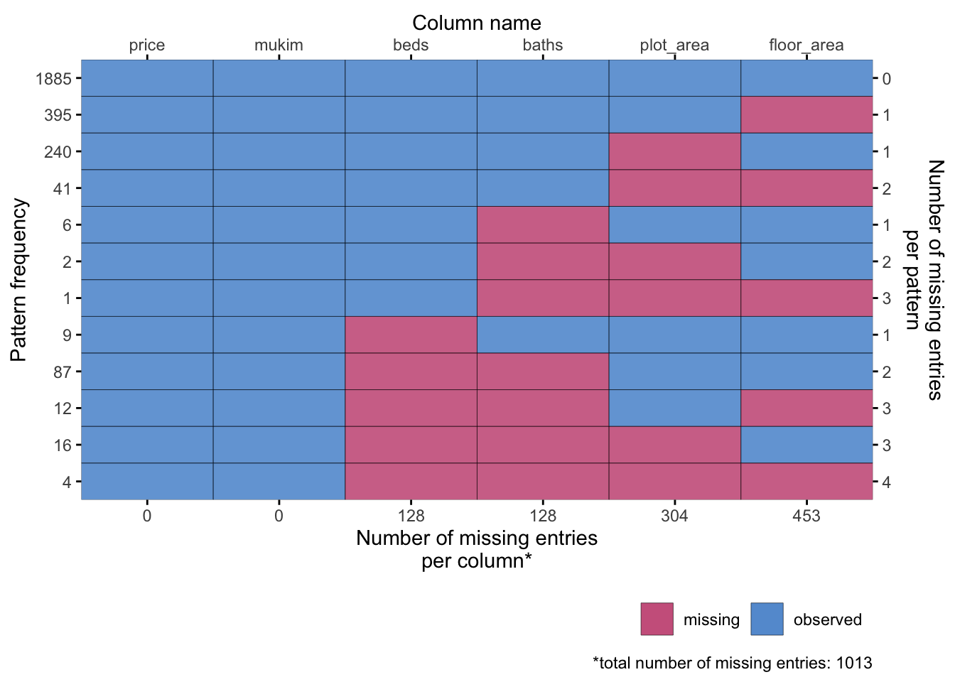
There are a total of 2698 houses in the Brunei-Muara district in 2024. There are a couple of missing values in the data set, 1013 to be exact. We can visualise this using the {mice} and {ggmice} package.
In [3]:
library(mice)
Attaching package: 'mice'
The following object is masked from 'package:stats':

    filter
The following objects are masked from 'package:base':

    cbind, rbind
library(ggmice)
Attaching package: 'ggmice'
The following objects are masked from 'package:mice':

    bwplot, densityplot, stripplot, xyplot
Let’s take a look at the missing data patterns in the housing data.
In [4]:
plot_pattern(hsp24, square =!TRUE, rotate =!TRUE)
We first note that in this instance, there are no missing values for price and spatial location. However, there is a pattern in the missing data, so the missingness mechanism is not completely at random. It seems to be the case that the missing data is at random (MAR), which means that the missing data is dependent on the observed data. We can test this using a logistic regression.
Call:
glm(formula = beds ~ plot_area + floor_area + baths, family = binomial,
    data = mutate(hsp24, across(everything(), is.na)))

Coefficients:
               Estimate Std. Error z value Pr(>|z|)
(Intercept)     -5.5048     0.3427 -16.065   <2e-16 ***
plot_areaTRUE   -1.0541     0.6745  -1.563    0.118
floor_areaTRUE  -0.5194     0.6731  -0.772    0.440
bathsTRUE        8.4491     0.5281  15.998   <2e-16 ***
---
Signif. codes:  0 '***' 0.001 '**' 0.01 '*' 0.05 '.' 0.1 ' ' 1

(Dispersion parameter for binomial family taken to be 1)

    Null deviance: 1030.18  on 2697  degrees of freedom
Residual deviance:  181.66  on 2694  degrees of freedom
AIC: 189.66

Number of Fisher Scoring iterations: 8
What we can see is that the beds variable missingness is dependent on the bath missingness, which means that if the number of bathrooms is missing, the number of bedrooms is also likely to be missing (odds ratio increases by \(e^{8.52} = 5014.1\)).
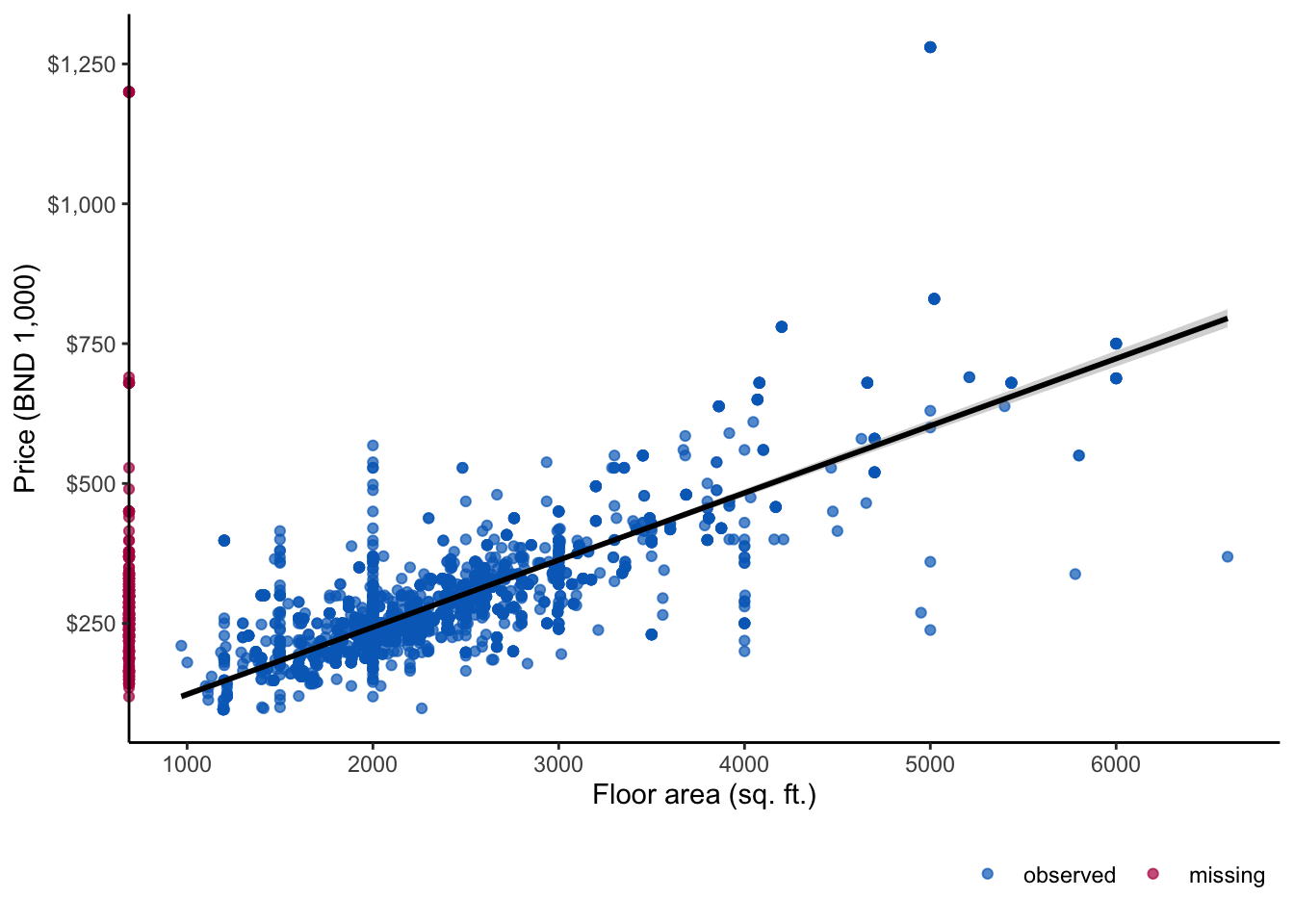
On the other hand, the missingness of the floor_area variable does not seem to be dependent on the other variables, which means that this variable is missing completely at random (MCAR).
# Step 2: Randomly sample from this multinomial distributionmis <-sample(x = pat$pattern, size =nrow(datB), prob = pat$prop, replace =TRUE)# Check that it matches the original patternround(prop.table(table(mis)), 3)
# Step 3: Introduce missing values into the complete dataset based on these proportionsfor (i in1:nrow(datB)) { na_flags <-as.integer(strsplit(mis[i], "")[[1]]) ==0L datB[, c("beds", "baths", "plot_area", "floor_area")][i, na_flags] <-NA}
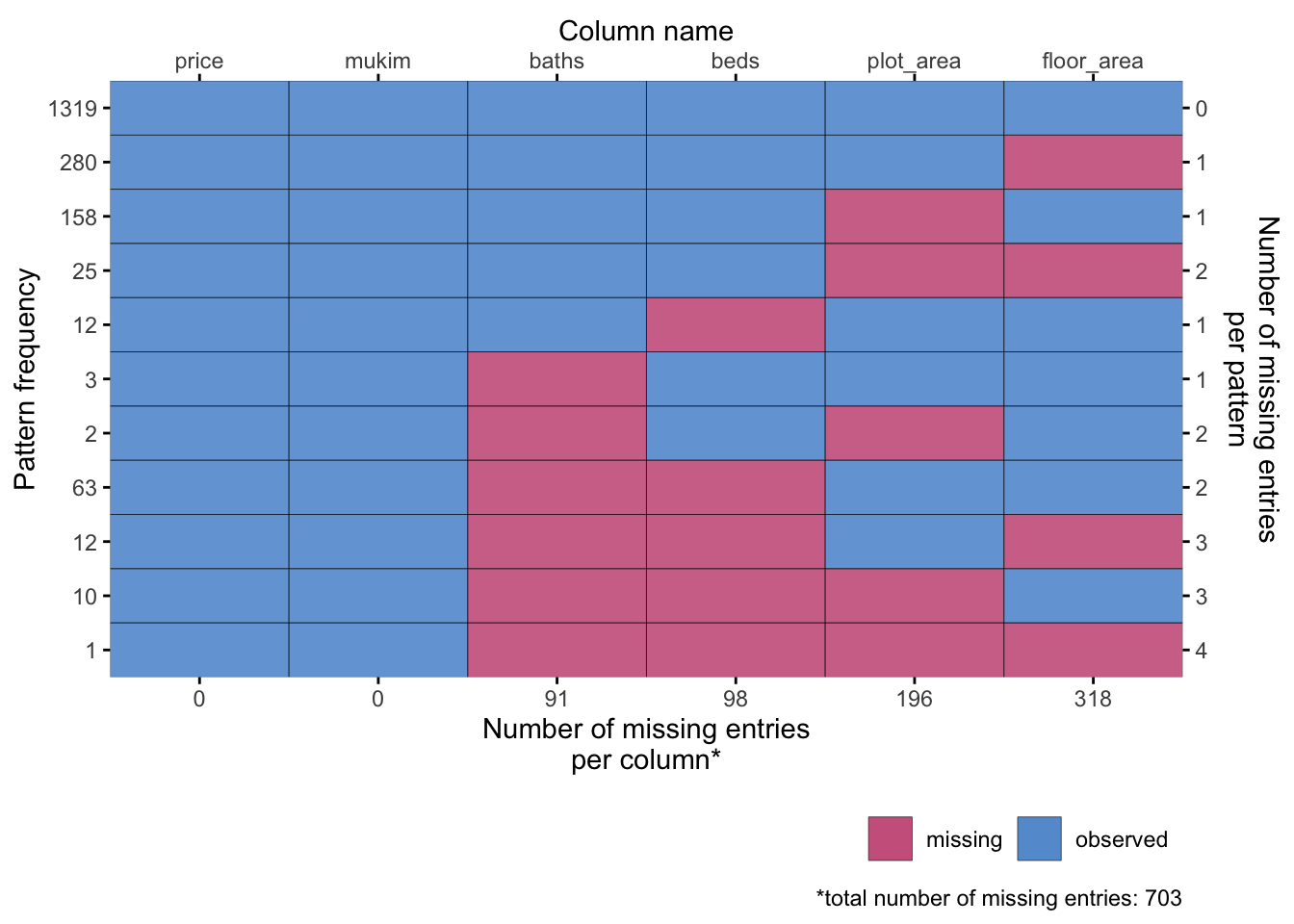
Let’s visualise the missing data patterns in the simulated data set.
In [9]:
plot_pattern(datB, square =!TRUE, rotate =!TRUE)
Some patterns are there, but some are not. This is expected when some of the missing patterns are rare.